Matrices

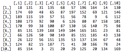
So far we have worked in only one dimension. Matrices are tables with two dimensions: It contains rows and columns:

IMPORTANT: Matrices can contain only one type of element: numeric or character (you will see the boolean later.. oops, a new word here :). All lines should have the same number of elements!

Below is how to create matrices:

> ## Creation of a matrix mat
> mat <- matrix(nrow=2, ncol=3)
> mat
> ## Creation of the matrix mat with values
> mat <- matrix(data=1:6, nrow=2, ncol=3, byrow=T)
> mat

Remark: 'matrix' is the second function that we see. 'data', 'nrow' and 'ncol' are called the parameters of the function.

Exercise 5:

• Create 4 vectors 'gene1', 'gene2', 'gene3', 'gene4' each containing 3 numeric values of expression
• Combine the vectors with 'c' and create a matrix 'matrix1' with each line containing a gene
• Define the row names of matrix1 with the function 'rownames' and the column names with the function 'colnames'

BAM! You have a matrix of gene expression in different conditions! Now is how to access and modify it:

> ## Access the expression value of gene2 in the third conditon (second row, 
> ## third column)
> matrix1[2,3]
> ## Modify the expression value of gene 3 in the second condition
> matrix1[3,2] <- 154
> matrix1
> ## You can also access the expression value using names!
> matrix1["gene3", "condition1"]

Powerful isn't it? Almost ready to perform your differential expression analysis!

Exercise 6:

• Access the values of gene 1 and 2 in the third condition using row and column names
• Do the same thing using numbers